Under development: this lecture is still being written and checked. Content may change.

Home › Teaching › Laboratory Courses › Uncertainty analysis

Still under development. The deck is a working draft and has not yet had the lecturer's full review. The tutorial sheet and the supplementary note will be added here when they are ready. If you find an error, please tell the lecturer.

About this lecture

Central question: how good is this number, and how do I show it?

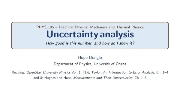
One lecture, taught over three contacts, on how to report a measurement honestly: with an uncertainty, correctly rounded, and compared fairly with theory. A single experiment, the simple pendulum measurement of g, runs through the lecture from sources of uncertainty to the final budget.

Reading: OpenStax University Physics Vol. 1, section 1.6; Taylor, An Introduction to Error Analysis; Hughes and Hase, Measurements and Their Uncertainties.
Learning outcomes

By the end of the lecture, you should be able to:

  1. Report a result as (value ± uncertainty) unit, correctly rounded, with its percent uncertainty.
  2. Distinguish accuracy, precision, random and systematic uncertainty, and classify a source as Type A or Type B.
  3. Calculate the mean, standard deviation and standard error of repeated readings.
  4. Propagate uncertainties through a formula and find the dominant source.
  5. Fit a straight line, interpret its residuals and χ², and report slope and intercept.
  6. Build an uncertainty budget and test agreement with an accepted value.

Three contacts

Understand, quantify, apply

Contact 1

Understand

What is a result, and where does uncertainty come from? Accuracy against precision, random against systematic sources, Type A and Type B, and reading an instrument.

Contact 2

Quantify

How do repeated readings and formulas give a number with an uncertainty? Mean, standard deviation, standard error, and propagation of uncertainty.

Contact 3

Apply

Graphs, budgets, comparison with theory and the report. Straight-line fits, residuals, the uncertainty budget and the test of agreement.

Physicist's Toolkits

Six reusable methods

  1. Reading an instrument
  2. Classifying a source
  3. Summarising repeated data
  4. Propagating uncertainty
  5. Linearising and fitting
  6. Building a budget and comparing results

Running example: measuring g with a pendulum

One experiment, from the first reading to the final comparison

A pendulum of length L = 0.800 ± 0.002 m is timed over 20 oscillations, ten times. The period is T = 1.795 ± 0.005 s, and g follows from

g = 4π²L / T²

The squared T counts double in the propagation, so the timing dominates the result. After the correction for the finite amplitude, entered in the budget as a systematic term, the deck finds

g = (9.77 ± 0.03) m/s²

Rule. Compare two results in units of their combined uncertainty. A measurement agrees with an accepted value when the discrepancy is small compared with that uncertainty. Round last.

The full working, including the contribution table and the comparison with the accepted value, is in the deck.

Laboratory sessions

Uncertainty analysis is shared by the laboratory courses PHYS 105, 106 and 205. The same methods for reporting a result, combining uncertainties, fitting a graph and comparing with theory apply in all three.

Hope Donglo leads the laboratory sessions for these courses. This lecture is the common support for the lab work. The deck below is available now; the tutorial and supplementary note will be added here when they are ready.

Open the deck (draft)

Files

All files are PDF

Deck (draft)Tutorial: coming soonSupplement: coming soonPractice questions: coming soon

Back to Laboratory Courses